Abstract
Thermoelectric coolers (TECs), also known as Peltier devices or thermoelectric heat pumps, offer numerous advantages, including the ability to heat and cool from a single device, bi-directional operation, and solid-state construction. However, because their performance parameters change with hot and cold side temperatures, accurately predicting TEC performance under dynamic conditions, such as thermal cycling, presents a significant challenge. This paper explores the limitations of traditional steady-state methods in analyzing TEC performance and presents a deterministic analytical approach using three custom-developed tools: a closed-form mathematical TEC model, custom thermal modeling software, and a simulated control loop. Together, these tools allow accurate performance modeling for dynamic thermal systems and enable selection of the optimal TEC device for a specific dynamic application.
Introduction
Thermoelectric cooling systems provide heating and cooling using a single, solid-state device. Among the advantages of TEC systems compared with conventional temperature control systems can be increased reliability, reduced vibration and electrical noise, compactness, and reduced cost. However, accurately predicting the performance of TEC systems, particularly under dynamic conditions, is not a trivial exercise.
TEC performance characteristics are a function of the hot and cold side temperatures of the device. Depending on these temperatures, a TEC could have its full heat pumping capacity, or have none. TEC datasheets include performance data at a few operating points, which is satisfactory for selecting a TEC model for steady state application, but not particularly helpful when trying to specify a TEC for a thermal cycling application. Designers are left to follow an empirical approach to selection, which may result in selection of a suboptimal device, and add time to the development schedule.
In this paper we explore an analysis technique which enables designers to deterministically predict performance of TEC-based systems, even in dynamic use cases.
Quick Refresher on TEC Operation
A TEC can be thought of as a bi-directional heat pump that moves heat from one surface of the device to the opposite surface. If one surface of the TEC is in contact with a cold block, and the opposite surface is exposed to a warm environment, by passing direct current through the TEC, you can cool the block further or reverse the polarity and cause the block to warm faster than it would have due to natural convection. This useful behavior makes TECs a natural fit for thermal cycling applications in biotech.
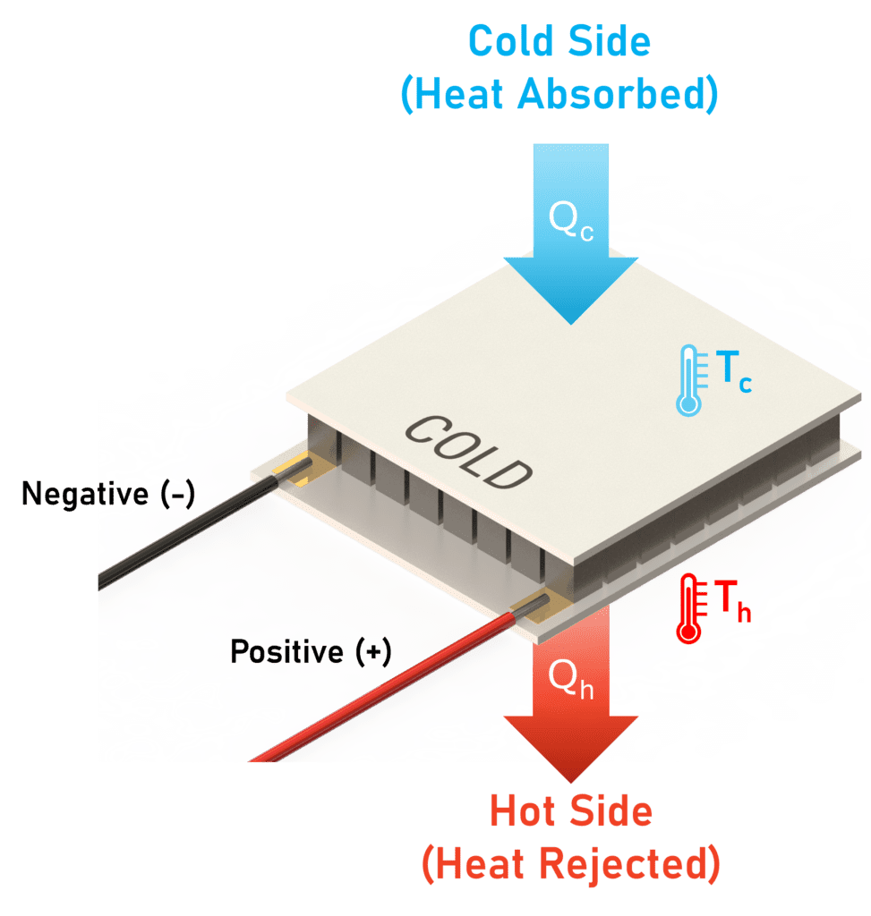
The terminals of TEC devices are color coded or marked to indicate positive (+) and negative (-). Some indication is also provided to identify the “cold” side of the TEC. When voltage is applied with the positive lead of the power supply connected to the positive terminal of the TEC, heat will flow from the cold side of the TEC device to the opposite (“hot”) side (see Fig. 1). Reverse the polarity and heat will flow in the opposite direction. The temperatures of the hot and cold sides are referred to in performance charts as Th and Tc respectively. Note that the direction of heat flow is dependent on polarity, and not on the temperatures of the hot and cold sides of the device.
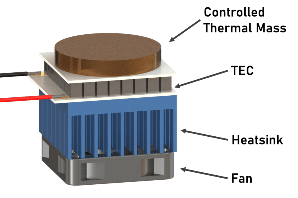
In cooling applications, TECs are incorporated into systems that include a thermal mass in which the temperature is controlled, typically attached to the cold side of the TEC, and a heatsink, typically with a fan to increase convective heat transfer, attached to the Hot side of the TEC to dissipate heat to the environment (see Fig. 2).
To maintain the thermal mass at a constant temperature, the TEC must remove heat from the thermal mass at a rate equal to the heat gain of the thermal mass from the environment (Qc). The TEC relies on the thermoelectric effect to generate its heat pumping capability.
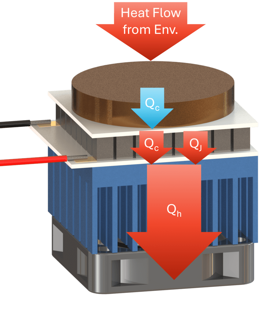
TECs rely on semiconductors to produce the thermoelectric effect, and semiconductors are resistive elements. During operation, semiconductors produce I2R losses, causing Joule heating (Qj) in the device. The Joule heating load Qj increases the heat load that will need to be rejected by the heatsink (Qc+Qj=Qh, Fig. 3).
A separate effect that diminishes the efficiency of TEC devices can be referred to as thermal backflow, which is conductive heat flow in the opposite direction of TEC operation. Thermal backflow is caused by the temperature difference between the two sides of the TEC. Thermal backflow can be largely ignored for steady state applications as it is baked into the manufacture’s performance data.
When selecting a TEC for a steady state application, the proper TEC model can be selected by referring to the manufacturer provided datasheets. Selecting the optimum TEC for dynamic applications requires developing a model of TEC performance that includes Joule heating, thermal backflow, and the thermoelectric effect.
Traditional Analysis for Steady State Situations
For steady state conditions, where the set temperature of the controlled thermal mass and the environmental conditions are constant, the selection of the most appropriate TEC element is a fairly straightforward, but iterative process.
The traditional process for estimating the performance of a Thermoelectric Cooling (TEC) system involves several steps. These can be briefly summarized as follows:
TEC Selection Steps for a Steady State Chilling Application
- Establish the set temperature of the thermal mass and the temperature of the environment.
- Calculate the heat transferred to the thermal mass from the environment (Qc).
- Select a candidate TEC model from the manufacturer datasheet.
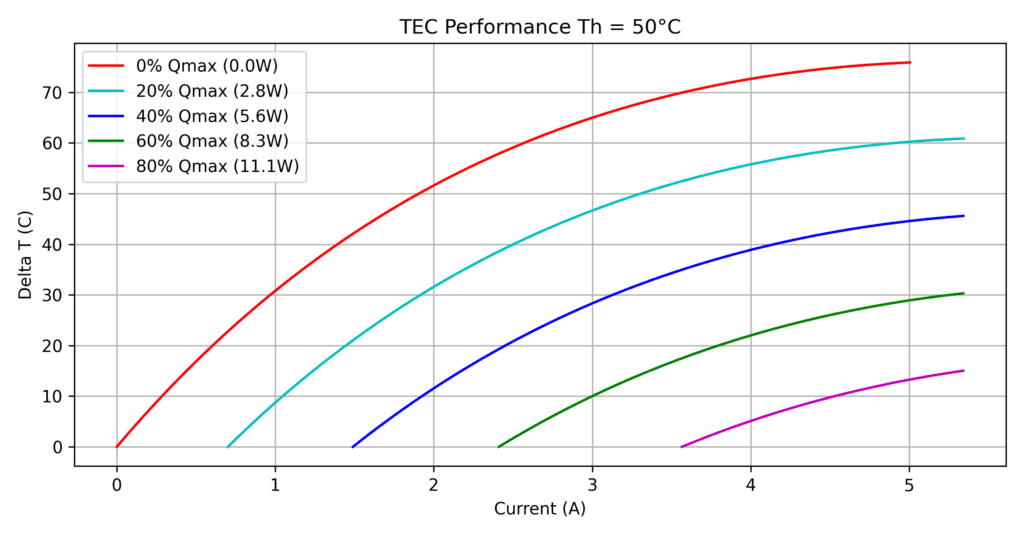
- Select a performance chart (see Fig. 4) with an appropriate Th (about 25°C above the environment temperature).
- Calculate temperature change across the TEC (ΔT).
- Interpolate the data from the performance chart to estimate the current (I) that corresponds to Qc.
- Calculate the Joule heating (Qj).
- Calculate Qh (Qh = Qc + Qj).
- Select a heat sink capable of rejecting Qh and calculate the heatsink temperature.
- Use the heatsink temperature as an updated Th.
- Repeat steps 5-10 n times until Th has converged and the heatsink and TEC have satisfied design constraints.
Dynamic Thermal Control Applications
The steady state process described above may be tedious, but it is possible to select appropriate TEC and heatsink components using manufacturer supplied data. In dynamic applications such as thermal cycling, the system temperatures are changing rapidly, which means the required heat flow is fluctuating rapidly. This means the heat that needs to be rejected by the heatsink is changing rapidly, which means the heatsink temperature and Th are changing, which means the performance of the TEC is changing. What is the temperature of the heatsink? Are we even using the right Th chart now? Is there a better chart for the current Th? What is the delta T? What heat flow is available at these temperatures.? With all the interpolation and layered assumptions, do we have any confidence in the system temperatures?
As one can see, the steady-state analysis techniques are inadequate to select the TEC and heatsink components for dynamic applications. Because of this, design engineers typically oversize the TEC and test the system empirically to understand performance. This approach is time consuming and there is no guarantee that the optimum TEC system components for a given application will be identified.
For most of our client projects, minimizing cost and reducing product footprint are priorities. Furthermore, a deterministic approach almost always converges more quickly than an empirical approach. For these reasons, we have developed a set of three tools that enable an analytical approach to TEC system design. We incorporate these tools into a custom software program we call TESS (Thermoelectric System Simulator) that allows us to accurately estimate performance in dynamic applications such as thermal cycling, avoiding unforeseen problems, additional revisions, and the costs and delays that come along with them.
Mathematical Model for TEC Device Performance
The TEC model is a closed-form model of the TEC based on the fundamental equations which determine heat flow in the TEC. By populating the model with datasheet parameters from multiple Hot Side temperatures, the model gains the ability to calculate the performance of the TEC at any combination of Hot and Cold side temperatures.
Discrete Time, Lumped Capacitance Simulator
The lumped capacitance simulator models thermal interactions in a system by treating components of the system as thermal masses interconnected with thermal resistances. The simulator uses steady state heat flow equations over very small discrete time slices. For each time slice the heat flows between thermal masses are calculated based on their temperatures and the resistances between them. The simulation then updates the temperatures of the thermal masses based on how much heat flow they received over the time slice. By repeating this process many times over very small time slices, the simulator can accurately model the heat flows in the system.
Simulated Control Loop
The last tool in NOVO’s suite of tools is a discrete-time control loop simulator. The simulator has all of the common elements of a control loop: P, I, and D gains, integral windup limiting, optional feed forward, etc. It takes an input file with commanded temperature values as a function of time and using the error between the actual temperature of the controlled thermal mass and commanded temperature applies the control law to drive the output to the plant (TEC).
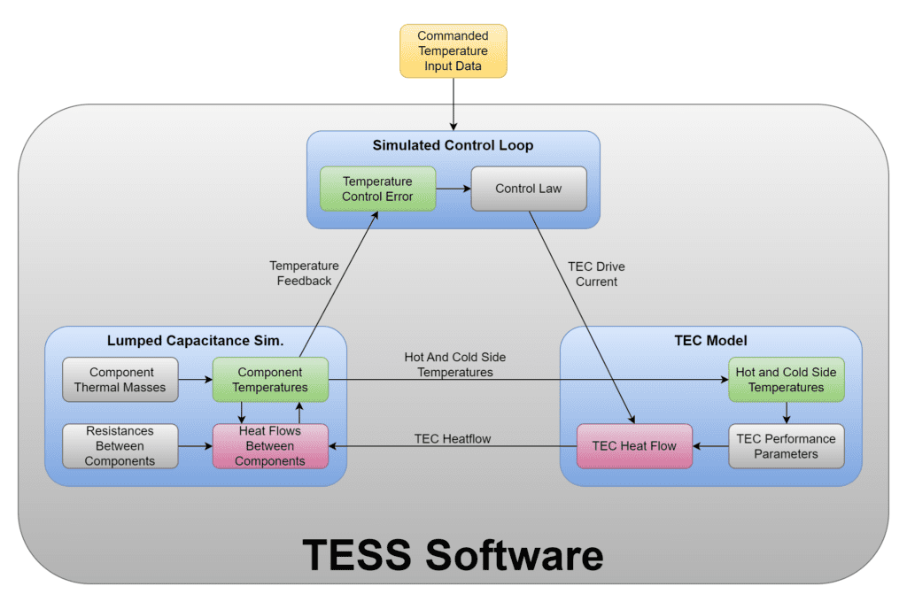
It’s when these three tools are combined in TESS that the true value of the tools is realized, allowing each to provide inputs to the other. During each time slice of a simulation, the lumped capacitance model updates system temperatures and heat flows between components, which enables updating the performance parameters of the TEC model, which enables accurate modeling of its heat flow given the control input, which is, in turn, affected by the feedback temperature that the controller sees. This complex system of interactions is shown in Figure 5. When simulated at tiny time intervals the tools continuously update one another to accurately predict system performance over extended periods of time, under highly dynamic conditions, thus providing a deterministic analysis of system performance.
Benefits of Utilizing This Approach
The benefits of using this approach when designing dynamic thermal systems are numerous. Instead of checking performance at a handful steady-state operating points, the TEC model can tell us what the TEC’s heat pumping capability is and how much is being used at any point in the simulation. We can literally understand how much margin our system has at every point of a ramp. Furthermore, we can easily swap in and out different models of TECs, enabling us to choose the optimal TEC for each project’s unique design constraints. We can also predict system behavior over many ramp cycles, helping to identify any other potential shortcomings in a system, all without building any hardware. The end result is ability to design dynamic thermal systems powered by TECs with much higher confidence in a design’s performance margin, while significantly reducing the probability for unforeseen issues leading to re-designs, schedule delays, and cost overruns.
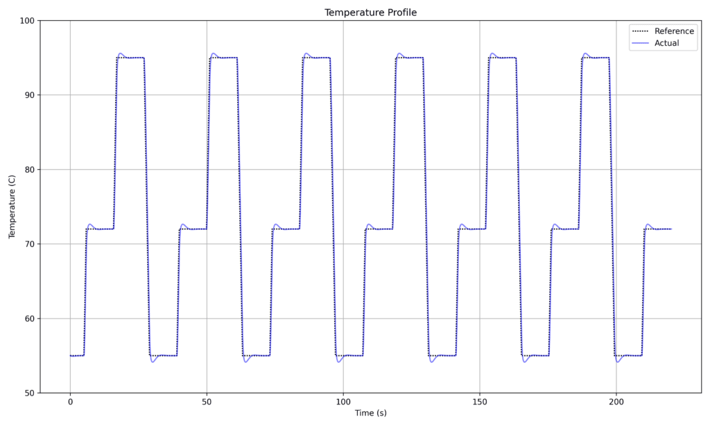
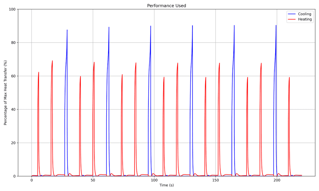
In the example below we can see a system running a classical PCR temperature profile, cycling between 55°C, 72°C and 95°C (Figure 6). The lumped capacitance model keeps track of system temperatures, the TEC model uses these to update the TEC performance and the control system drives the simulated TEC to pump heat into the simulated system. Throughout the simulation, the percentage of heat pumping capacity being used is recorded by the modeling software (Figure 7). This powerful tool allows us to see our TEC’s design margin throughout the entire temperature profile. This is something that simply can’t be done with steady-state tools. Looking at the plot, we can see the usage during downward ramps is ~90% of maximum cooling. This tells us we have minimal margin (only 10%) at these ramp rates. We are pushing the TEC about as hard as is prudent. If there is any possibility that marketing could add use cases with higher ramp rates or we want a highly robust system with plenty of margin, we should consider designing in a more powerful TEC now to avoid all the issues that come with making late-stage design changes. The ability to gain these types of insights is just one example of how NOVO’s suite of TEC analysis tools can be used to deterministically analyze system performance, thus reducing risk and enabling system optimization without building any physical hardware.
Conclusion
TECs offer numerous benefits, but accurately predicting their performance under dynamic conditions can be challenging. Limited data provided by manufacturers and the complex interactions between system temperatures and TEC performance make it difficult to analyze TEC performance in highly dynamic systems. NOVO has integrated a set of proprietary thermal analysis tools into TESS, a program that enables deterministic analysis of TEC performance. TESS offers streamlined development for high-performance thermal cyclers for our biotech clients.
In conclusion, deterministic engineering analysis enables a more accurate and comprehensive evaluation of TEC-based thermal systems. By utilizing the TEC model, discrete-time dynamic lumped capacitance modeling, and control loop simulation software, engineers can confidently predict TEC performance in dynamic conditions, reducing risk, preventing costly redesigns, and facilitating faster development of future TEC applications.